The danger of failing to interpret the predictions of your machine learning models
In recent months, BBVA Next Technologies has devoted some effort into researching tools and techniques for interpreting machine learning models. These techniques are very useful to understand the predictions of a model (or make others understand them), to extract business insights from a model that has managed to capture the underlying patterns of customers interest, and to debug models in order to ensure they make the right decisions for the right reasons.
In this article we will explain how we have applied these techniques to avoid deploying flawed models into production that seemed totally correct a priori according to standard validation methods.

A Brief Introduction to Interpretability
Machine learning models are an extremely powerful tool for solving problems where there is enough data available with the required quality. Nowadays this tool is used in a large number of fields, many of them of great relevance to our lives, such as medicine, banking or autonomous cars.
One of the main problems with these models is their high degree of complexity, which makes it very difficult to understand directly why a model makes a decision. Since we are talking about important decisions, there is a need to find ways to understand, even roughly, what a model is doing. In this context, in recent years a set of techniques has emerged (or resurrected) that allow, in greater or less detail, to understand what an machine learning model is doing.
In addition, from the point of view of the data scientist, there is an additional reason to use interpretability techniques: validation and debugging of models. As shown below, many of these techniques can help us find critical errors in our models or our data quickly and easily, thus avoiding possible unexpected results.
Case Study: Car Damage Detection
A few months ago we conducted a proof-of-concept on detecting car damage from images. We found it a very interesting problem, both for its straightforward application to real-world use cases and also technologically, since the complexity of the problem is high, and this would allow us to apply with purpose technologies close to the state of the art.
We found it particularly interesting to work with low quality images, such as those that can be obtained with a mid-range mobile device. This increases the difficulty of the problem, but also opens the door to more practical applications.
Would we be able to determine whether or not a car is damaged? Could we refine and locate the damage (for example, be able to see that the damage is in the right front side)? Could we even determine the magnitude of the damage (severe, medium, or mild)?

Fig. 1: Car damage detection use case (source)
The challenge was really complex due to two main problems:
- The great variability of car models and possible damages, as well as light conditions, car pose, etc.
- The poor quality of the images, being pictures taken by users with their mobile phone.
We spent the first few days of the project investigating whether someone had already solved the problem. We found several papers that approached the problem from different points of view, and we came across an open source project that claimed to solve it with excellent metrics. We were quite skeptical about the claimed results, but just in case we jumped to check if it was true.
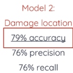
Fig. 2: Metrics published by the open source project neokt/car-damage-detective
The model used in the project to detect whether or not a car is damaged (binary classification problem) is a deep convolutional network with VGG-16 architecture. Ting Neo, author of the project, used the weights of a pre-trained network in Imagenet, replacing the three final layers with two fully connected layers with dropout (0.5).
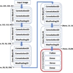
Fig. 3: VGG-16 architecture (source)
So we got down to work. We downloaded the related data set, replicated the model (damaged or undamaged car) correcting small bugs and, surprisingly, the metrics were very similar to those published by the author. But something didn't add up. The problem seemed extremely complex, and the solution too "simple". So the next step was to validate the model in our data set. The result was amazing - the metrics in our dataset were even better!
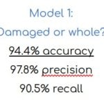
Fig. 4: Metrics obtained with Model 1 in our data set
What was going on? We might have overestimated the difficulty of the problem. And it was really good news. We had solved the problem in a very short time. But before singing the praises, we decided to use interpretability techniques to check which parts of each image the model was "looking at" to decide whether or not a car was damaged. If the model was correct, it should look at the damaged parts of a car to make the decision as to whether or not it is damaged.
In this case we decided to use LIME. LIME (Local Interpretable Model-agnostic Explanations) is an interpretability tool that can be used in any classifier based on machine learning. LIME allows to give an "explanation" of any prediction of a model in the form of a linear model with few features. Specifically for the case of models whose input are images, LIME creates superpixels of the input image and "turns on and off" each superpixel to check its influence on the final prediction. This way, it estimates which superpixels have had the most influence (positive or negative) on each prediction.
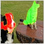
Fig. 5: Example of LIME explanation for a classification model for dogs and cats. In this case, the prediction of the model is "cat". LIME indicates in green the most positively relevant superpixels for the prediction, and in red the most negatively relevant (source).
Although we have reservations about LIME because of its inconsistency under certain circumstances, the official implementation is good, easy and quick to use.
So we downloaded some car images from the internet, passed them through the model and used LIME to see what the model was focusing on. Below are two example results:
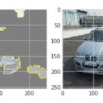
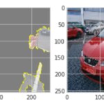
Fig. 6: Examples of interpretability results using LIME, car images and the model to evaluate. As you can see, the model is mainly looking at the environment, not the car.
As the image shows, the model was primarily looking at the environment, not the car, to detect damage to it.
A review of the data sets clearly showed the problem. Most of the images labelled as "undamaged" vehicles in both datasets were brochure images, with pristine cars circulating in idyllic and retouched environments (beautiful mountain roads, a sunset on a coastal road...). In contrast, images of damaged cars showed more mundane environments: garages, car parks, people around the car and other cars in the background. The model had learned to classify environments, distinguishing between catalogue environments and environments closer to the real world.
Testing our hypothesis was simple. If the model classified environments instead of cars, it had to poorly predict all undamaged cars found in everyday environments. So we did a final set of tests with images of undamaged cars in non-idyllic environments. The model predicted that all cars were damaged, confirming our hypothesis.
Applying interpretability techniques took a couple of hours and solved our doubts about the model. This case may seem obvious, and surely we would have reached the same conclusion by spending more time analyzing the data set. But in many other cases the problems are not so visual, and it is much more difficult to realize that your model, which is apparently good, is actually a disaster.
Had the model been put into production in the aforementioned use case, the vast majority of cars would have been labeled as damaged by the application. Others, damaged but in more beautiful environments, could have been classified as undamaged. The model would have completely failed.
Case study: Predicting sales in new stores
John works for a retailer. He is one of the people responsible for finding new locations to expand the network of establishments. Fortunately, John has a tool that helps him better understand the sales potential of each store. When John sees an empty premise in a neighborhood of interest, he comes closer, takes out his mobile phone, opens an application and clicks the "Estimate sales" button. The application sends the coordinates of the phone to a set of machine learning models that, based on socio-economic information of the environment, historical data and competition data, estimate the annual sales of the potential new establishment.

Fig. 7: Estimate of the areas of influence of an establishment
The previous paragraph summarizes the use case we had to solve for a retail client. One of the first versions of the model obtained very good metrics in the test data. Many expectations had been generated about the application and there was some pressure to accelerate its development. Fortunately, we decided to invest some time in applying interpretability techniques to the model to check that the variables on which it based its predictions made sense from a business point of view.
The model is actually a "waterfall of models", all based on trees. The first layer of models generates features that serve as an input to the second layer, which is the one that makes the final sales estimate.
This time we decided to apply ‘Permutation Feature Importance’, a technique that allows us to know the importance that a model gives to each variable globally. The result was the following (variables have been grouped by category to simplify the table):
Fig. 8: Summary table of feature importance for the main model
The most influential variables in the predictions of the model were the characteristics of the hypothetical business premises (size, average price of the products,...). Since the business premises does not yet exist when the model is used, these characteristics are chosen by the expert. Surprisingly, the prediction was similar for the center of a large city than for a small town. Why did the socio-economic environment or the presence of competition hardly matter for our model? Why did the sales estimate of any of the business premises with a specific configuration not vary significantly depending on the location?
Reflecting on the result and on the process to obtain the data, we clearly saw the problem. The experts choose the characteristics of the shop according to the environment, the competition and their own estimation of sales for that shop. For example, if an expert considers that a shop is going to sell 1M€ per year, he will choose a smaller premises than if he considers that it is going to sell 10M€ per year. In our data set there is an implicit relationship between the characteristics of the shop and the expert sales estimate. The model detected this relationship and took advantage of it. Therefore, we had a model that always proved our expert right. As long as the expert introduced inputs with judgement, the model would have given a good estimate.
But what would have happened if we had put this model into production? The experts would start to trust the model, because it worked apparently well. At some point, an expert who relied on the system would start experimenting, and see that huge stores with very high rates have fabulous sales predictions. The expert would then place business premises as large as possible, regardless of the environment. The results, of course, would be economically catastrophic. Huge shops would be opened in small towns expecting big profits erroneously.
The solution in this case was as simple as removing the variables containing expert information from the model input. The apparent precision of the model was reduced, but now we had a model that truly fulfilled its mission.
Check it out for yourself
A few months ago we prepared a training session for Big Data Spain which included an interpretability module. In that session we proposed to the assistants to solve the mystery that we explain below (whose solution can be found in this notebook).
First we downloaded a public set of image data of dogs and cats, containing 25000 images of tagged dogs and cats. We wanted to introduce a bias into the data set that was simple and not too obvious. So we selected darker images of dogs and lighter images of cats from the data set.

Fig. 9: We used the Kaggle Dogs vs Cats dataset (source)
Although this bias can be detected relatively easily in a detailed exploration of the data set, we found it subtle enough to serve our purpose.
Once a new biased data set was obtained, we trained a simple CNN that (surprise!) was able to distinguish dogs from cats with 100% accuracy (you can see the model training in this notebook).
The challenge was that participants, without knowing the bias introduced in the data a priori, tried to detect what was failing in a model that, apparently, was perfect.
Using SHAP, another great tool for interpreting models, participants could easily obtain results that showed the problem in the model (and in the data).
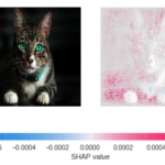
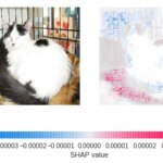
Fig. 10: To the left, the images that were presented to the model. To the right, the estimate of the SHAP value for each pixel. Higher values (pink) indicate that the pixel contributes to the prediction being "dog". Lower values (blue) indicate that the pixel contributes to the prediction being "cat". Values close to zero (white) indicate that the pixel hardly contributes to the final prediction.
As can be seen, in both cases our model is almost completely ignoring the cat, our protagonist, deciding whether or not the image belongs to a cat by observing almost exclusively the environment.
Conclusions
As shown in the three previous examples, a small investment in interpretability can significantly increase our confidence in our models before putting them into production. The cost is very small and the benefit can be enormous.
Do interpret!
Thanks to Jorge Zaldívar for his contribution to the supermarket sales example.