Teaching Business to our AI, a practical case
Cost and revenue factors impacting economic activities are often too complex to be properly modelled, in which case optimization through Artificial Intelligence (AI) can lead to academically correct solutions that fall far from being economically optimal solutions.

In this post, an effective business metric is constructed for a real case based on an unquantified reference of previous business performance. The new methodology compares new AI models and identifies the economic optimum, whether or not it yields the most accurate predictions.
AI Innovation Labs - Project team:
Alberto Hernandez Marcos, César Gallego Rodriguez, David Suarez Caro, Emiliano Martinez Sanchez, Enrique García Pablos, Gema Parreño Piqueras, Germán Ramos García, Jerónimo García-Loygorri, José Luis Lucas Simarro, Leticia García Martín
This article in 1 MINUTE!
Problem
- To improve an old "product recommender" with Machine Learning...
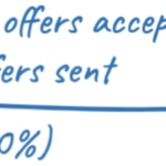
- Based on its results to date (accepted / rejected offers)...
- Ignoring the accurate cost/benefit drivers (e.g. cost of sending an offer)
Methodology (simple version)
1. Assume the old model hit break-even
2. Estimate revenue / cost q ratio based on it
- 3. Train new models from past results (e.g. supervised learning)
- 4. Now apply q ratio to each model’s results and...
- 5. Estimate the % of Theoretically Achievable Profit* they actually get!
*i.e. if offers were only sent to the customers that will accept them (ideal case).
Results
In real cases (like the one here) the model that "predicts better" is not always the most profitable one.
Instead, a new business metric (RAP) is proposed based on the methodology above.
The new metric doesn't require accurate cost/benefit drivers, but a previous baseline of predictive performance.
Introduction - The problem of comparing AI models
The development of Machine Learning projects involves a design phase in which different models are trained from data, tested and compared before its deployment into production. Often very different paradigms of AI (Artificial Intelligence), software libraries, frameworks and data transformation strategies are tried, but in the end a single concrete metric must be applied to all the models for an objective comparison that points to the best.
If it is about intelligence, why not choose the model that "predicts better"?
Well, that is not always the best choice... In principle, the more similar the predictions of a trained model to the real values expected in our data, the more valid it will be (in the context of supervised learning). However, comparing AI models by their predictive power (precision, ROC curve ...) can lead to deception in real business cases. The reason is that the cost-benefit ratio of predicting the desired class (a real emergency, a suitable client) is not comparable to the failure (a false alarm, an uninterested customer). In addition, taking into account that these events are usually imbalanced (there are more cases of one than of another), the problem is exacerbated.
Think of an alarm system: the cost of investigating an ultimately dismissed emergency is usually much less than the damage caused by an unidentified accident. In a different field, such as marketing, the comparison could be applied between the cost of a wasted advertising delivery and the profit lost from not identifying a willing customer. In both cases, the relative importance of predictive errors is very uneven.
For this reason, the metric finally chosen may not necessarily be of a "cognitive" nature (rates such as accuracy, precision, F-value ...), but one summarizing the business priority for the use case (e.g. maximize the return on investment). In general, this can be accompanied by additional requirements to be satisfied by other metrics (e.g. maximum acceptable latency in response time, acceptable limits for certain equity metrics or "fairness", etc.).
In summary, the actual model chosen will be the one that maximizes the selected metric, which if it is of a financial nature, will not necessarily yield the maximum predictive rate.
Ok, would it be a matter of weighing these costs / benefits on the predictions then?
In theory, yes; In supervised learning (where we have labeled samples of the results we expect from the model), we can balance the successes and failures weighted by the given values. However, in practice, for very different reasons, organizations are rarely able to provide real and reliable quantifications of these values. One of the main reasons is the difficulty of estimating the indirect costs or benefits of an action taken, beyond those directly associated.
This article proposes, on a real practical case, a simple methodology for the comparison of AI models based on business metrics. The proposed metric only requires a base line of previous performance not quantified economically.
Real case study: event-driven marketing
We will illustrate the methodology with real data from a proof of concept carried out in the field of "event-driven marketing", where the objective of an AI recommendation model is to predict in real time which clients are likely to accept the offer of a certain product, which triggers the delivery of the offer.
In this case, we will financially compare different AI models against a baseline of the predictive (non-financial) performance of the previous model in use.
Original scenario
The system prior to the training of new models included:
- A system (already in production) that received all card operations as real time events (purchases, cash extraction, deposits).
- A rule-based AI system that recommended in real time appropriate financial products based on the information of the event (a card transaction) and on historical data about the client.
- A data collection system that recorded all the activity during a certain time interval: events received, offers sent and final result of each offer sent.
The objective of the proof of concept was to validate whether a new recommendation model could be trained by means of machine learning, as an alternative to the rules systems, to give an equivalent or better performance. The reason is that rule-based systems often require very expensive maintenance and their performance decreases when the number of integrated rules is high.
Performance baseline
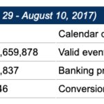
After monitoring the system for little more than two months, a volume of hundreds of millions of customer card events was recorded, for some of which the rule system triggered the sending of offers, and a high percentage of the events triggered no offer.
The focus of the proof of concept was on one of the banking products offered, showing the largest volume of data and a relatively balanced success rate (2.79% success rate, which is within retail marketing standards). [It is common in areas such as marketing or security that the "positive" class sought (eager clients, fraud cases) occurs much less frequently than the other, which is known as class imbalance]:
This is the available ground truth on the performance of the existing rule system. However, accurately quantifying this performance in business terms would mean estimating values for the full underlying business model (shipping costs, indirect costs, opportunity costs due to channel saturation, revenue by type ...), which would have led to an unmanageable complexity. Instead, a new methodology was tried out.
Machine Learning Models
Different strategies were followed for the preparation of data and the training of models on the training set of some 148,837 samples of offers labeled as accepted / not-accepted, of which:
- 126,087 samples were used for training.
- 22,750 samples were separated as a test set on which to compare yields.
A total of 2,266 models were trained over three "generations", which were evaluated against the test set:
- 18 manually trained models, following different approaches (logistic regression, decision trees, support vector machines, etc.).
- 2,212 models of artificial neural networks automatically trained through hyper-parameter tuning.
- 36 logistic regression models automatically trained through a single hyperparameter tuning (number of features to use, prioritized beforehand).
For more details on the models, see "Appendix 2. Summary of trained model".
In addition, the following dummy or baseline models were included in order to validate the results of the trained models: predict-always-positive, predict-always-negative and predict-random-50%. (Trained models are expected to give better results than dummy ones.)
A methodology for the financial comparison of models
For the comparison of trained models beyond their cognitive capacity, we wanted to know their estimated impact on the business compared to the previous model. Not having a realistic quantification of the possible cases, but its success rate, the following methodology was established:
- Given the results of the pre-existing model, estimate the average cost / revenue ratio per offer sent / accepted based on a reasonable hypothesis (e.g. a break-even situation, in which the return on investment = 0%).
- Express the maximum Theoretically Achievable Profit (TAP) in terms of average unit cost and revenue. (In our case, TAP would ideally be reached if a single offer were sent to each customer who is prone to accept it, and all are effective.)
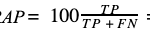
- Define the RAP metric (from Relative Achieved Profit) as the percentage of the TAP actually achieved by a certain model. Then, apply it to the results of each new model evaluated, selecting the highest among all.
1. Estimation of the average cost / revenue ratio based on a hypothesis of previous economic performance
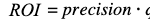
Ignoring the exact values of unit cost and revenue for all offers sent and accepted, a reasonable hypothesis about the Return on Investment (ROI) achieved by the preexisting model can be formulated, for example:
Hypothesis:
"The previous model recovers the investment exactly (point of 'break-even')". This means that ROI = 0.
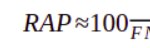
In general, knowing the results of the previous existing model
- TP=True Positives (number of offers sent and accepted)
- FP=False Positives (number of offers sent but not accepted)
- TN = True Negatives (number of unsent offers that would not have been accepted)
- FN = False Negatives ( number of unsent offers that have been accepted)
and being our unknown economic values
- c = average cost of sending an offer (unit cost)
- r = expected average revenue for an accepted offer (unit revenue)
the ROI can be expressed as follows (for the details on formulation, see "Appendix 1. Estimation of the ratio between unit revenue and cost as a function of ROI"):
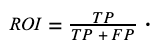
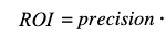
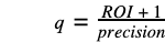
The first fraction represents the model's precision, and renaming the ratio between unit revenue and cost, or unit profitability, as q:
In our case, the values of TP and FP of the previous model yield an accuracy of 0.027856, so for ROI to be 0 we have:
q = 35.8989387
That is, the average revenue for each accepted offer must be about 35.90 bigger than the total cost of sending each offer. This means that if, for example, the unit cost c associated with sending an offer were $1.0, the expected average revenue r to cover costs exactly would be $35.90.
Other hypotheses about the performance of the previous model, for example, a moderate performance with ROI = 10%, would yield different values of q, which could impact the comparison of models. This effect is studied in "Results" below.
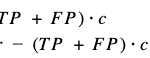
2. Express the maximum theoretically achievable profit for a model (TAP) based on the average unit cost and revenue
Given the results collected by a new model, tried on a certain test set, the maximum theoretically achievable profit (or TAP) would ideally be achieved if the new model sent an offer to each customer who was inclined to accept it (as collected in the history of the previous model), and none were sent in vain. This ideal coverage would include the successes of the new model (TP) plus those that should have been found, or false negatives (FN). The profit of each case would be simply the revenue minus the cost:
3. Define the metric RAP as the percentage of TAP obtained
Hypothesis:
We assume that the values of revenue and cost of the samples in the data set follow uniform distributions in which r and c are the average revenue and cost respectively.
According to this premise, each new model will yield non-optimal results according to this expression for profit (or P):
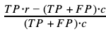
We can now express the percentage of the maximum theoretically achievable profit actually achieved by the new model, defined as RAP.
The equation, after some transformations, can be expressed as follows:
where:
TP, FP y FN are the results obtained by a new model on a test set (True Positive, False Positive and False Negative),
q is the ratio between unit revenue and cost estimated on the initial hypothesis.
The expression obtained only depends on the q value estimated and the results of the evaluated model. It is now possible to apply it to the results of each new model to be evaluated, choosing the highest one.
Discussion and selection of business metrics
Main metric: RAP
The main metric selected for the real case was RAP (Relative Achieved Profit) for the following reasons:
- 1. It provides an evaluation of the economic potential of each model independent of the number of samples, assuming that the proportions of false and true positives and negatives is invariant to volume.
- 2. It is bounded for optimal cases regardless of unit profitability:
-
- a. Maximum achievable profit: FP = FN = 0
RAP = 100% regardless of the ratio q.
-
- b. Maximum precision: FP = 0
- that is also independent of the q ratio. The result is limited to the value of the recall of the model, possibly giving very little real profit.
- 3. Its null value is consistent with the expected profitability of a model with the lowest possible precision, that is, with TP ≈ 0.
- which will be negative (economic loss) under the reasonable assumption that q > 1, that is, that unit revenue is greater than the unit cost.
- 4. Since the function is monotonically increasing and bounded between meaningful values, it allows the comparison of models tested on different data samples, assuming that their statistical distribution is the same.
ROI metric
The Return on Investment metric or ROI, despite meeting the same generality requirements as RAP, was not prioritized because its values do not directly indicate the volume of financial profit. A very cautious model (sending a few very well-targeted offers) with a very high ROI percentage does not necessarily outperform another that obtains a higher net profit at the expense of lower precision and ROI values.
Example:
Model B), despite having higher ROI, will yield less profit because it collects a smaller fraction of the maximum achievable profit TAP:
q = 35.90 [hypothesis: the previous model covered costs (break even)]
P Metric
Finally, the metric P (Profit) was not prioritized because its quantification required the values of the unit cost and revenue, which are not always precisely known due to the hidden associated costs. In addition, its value spans between 0 and the volume of each specific test population, not allowing between models from different samples.
During the exploration, scenarios were actually calculated on the hypothetical basis of $1.0 / $35.90 for unit cost / revenue, but their value and magnitude were only illustrative and contextual to the samples of the test set used, which did not provide the comparative generality of a percentage.
Results
AI metrics used
Cognitive metrics
They measure the predictive power demonstrated by AI models during their training and testing (or during their operation in production, once it occurs). In our proof of concept the following metrics were collected:
- Accuracy
- Precision
- Recall
- Probability of False Alarm
- Specificity
- F-score
Business metrics
They measure the economically quantifiable results obtained by the predictions of a model. In our proof of concept, the following metrics were calculated according to the methodology described above:
- Relative Achieved Profit, RAP [Main metric]
- Return on Investment (ROI)
- Profit P (scenarios on hypothetical values of unit cost / revenue)
Other metrics not used
There exist other possible dimensions or AI metrics that can be applied to trained models, such as:
- Ethical metrics, to ensure an acceptable and reliable performance of the AI according to a certain set of values or principles. An example is equity metrics, or "fairness", such as the one used in Alphabid, a real internal reference applied to ethical dynamic pricing.
- Computational metrics, measuring technical performance and consumption of infrastructural resources, for example: consumption of processing power, memory and network resources, data storage, latencies, etc.
In the current proof of concept, without an immediate goal of productionizing the model, the focus has been on carrying out a detailed analysis of the balance between the cognitive metrics and business metrics rather than all the possible metrics.
Models benchmarking
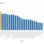
Cognitive metrics were collected from all the trained models and their results were used to compute their respective business metrics. The table below reflects the ranking by the main metric (RAP) of the most representative models trained plus some metrics of the baseline models, highlighting the maxima obtained in each metric. It can be seen how the most profitable model is not necessarily the best trained.

Ranking of some trained models according to the main metric RAP (% of the maximum achievable profit). Hypothesis: Previous ROI = 0%. The best trained model is not the most profitable one

Conclusions
Relevance of business metrics
- In the real case explored it would be impossible to identify the optimal model without the business metrics.
The highest percentage of the achievable profit is not obtained by any of the models with better cognitive results (precision, recall, F-score...), but by the one that appropriately weighs the effect of the predictions' successes or failures. Results show how the top-ranking model according to the RAP business metric beats the profitability of the one with the "best predictions" by 5% (from 25.7% to 30.7%).
- Despite its significance in the financial context, Return on Investment (ROI) cannot replace the main metric (RAP).
- Cognitive metrics are necessary during model training, although their comparative capacity is generally limited in real business cases.
Robustness of the initial hypothesis: "the initial ROI was zero"
The baseline hypothesis about ROI on which the q ratio was estimated is arbitrary and may be questionable; in general, ROI is expected to be higher than the 0% we assumed. For that reason, the effect of different hypotheses on the models ranking for our particular case was explored and the stability of the methodology verified.
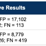
The graph below shows a sensitivity analysis with the RAP of each trained model resulting from the ROI assumed, highlighting the validity range of the chosen model.
Sensitivity analysis: Exploration of the RAP for each model as a function of the ROI assumed. The selected model remains optimal within a very wide range of hypotheses.
The conclusions drawn are:
- The methodology provides stability in the real case tested. The selected model remains optimal for hypothetical baseline ROI between -15% and + 50% approx., a very reasonable safety range for previous performance guessed.
- For ROI < -15%, three of the manually created models yield better economic results.
- For ROI > 50%, in which the unit cost is very low in relation to revenue, worse discriminating models prevail, with the "dummy" model that would always send an offer standing on top.
About the models training
- "The machine wins": The optimum model arose from the automatic design tool, despite the time spent designing and calibrating models manually, many of them based on the same winning algorithm (Logistic Regression). The application of automated hyperparameter tuning seems mandatory to achieve optimality.
- More complex models, such as neural networks, were trained automatically without the use of regularization, which is why they may have lagged behind simpler models. The inclusion of regularization hyperparameters in the automatic design tool (L2, dropout ...) would surely improve the results in this proof of concept.
- "Failure was cheap": despite its low predictive results, the performance of the "dummy" baseline model that always proposes to send is not easy to overcome economically; the reason is the high imbalance between the values attributed to offers’ cost and revenue. (Obviously the “dummy” model is not applicable in practice, since it does not take into account resource limitations or the saturation effects on clients.)
Feasibility of training a new recommender
- The proof of concept empirically confirms the feasibility of training a new recommendation model through Machine Learning with a predictive capability comparable to that of the existing rules system.
- Furthermore, in spite of the lack of knowledge about the unit cost and revenue values, it is confirmed that the new model would have a comparable economic performance at least, on the hypothesis that the previous ROI was between -15% and + 50% (with reasonable alternatives for the rest of cases). In fact, adding the economic prioritization provided by the model selected through this methodology, it becomes more profitable than the original rules system.
Limitations and next steps
First, although the results confirm the feasibility of Machine Learning for the use case explored, a rigorous comparison between the old rules system and the new models is not possible. The reason is that the results of the former were obtained on the general population of clients, and those of the latter on the subset of clients preselected by the rules, with different statistical distributions. A continuation of the proof of concept would involve the deployment in production of new models for real testing and progressive retraining.
Regarding the new methodology followed, the new business metrics were applied to the results of the new models trained. Instead, an interesting approach would be to integrate the new metrics directly into the training, for example by defining weighted cost functions according to the q ratio (or unit profitability). The objective would be to obtain q-optimal models directly from the training.
In more general terms, although the new methodology applied to this real case adds great value over the classical cognitive AI metrics, its stability with respect to the initial hypothesis in other use cases is not proven. We hope to learn more in future explorations on new data.
Finally, the hypothesis assumed regarding revenues and costs is that they follow uniform distributions, which allows applying their mean values to predictions. In cases where this doesn’t apply (for example, if they follow a normal distribution), the formulation would require a generalization that yields probability ranges, or a training process with individualized costs per sample. An interesting case could be fraud detection, in which the money amounts at risk in each evaluated operation show a high variance.
As for new possibilities following from this line, an approach that could enrich model choice might be the generalization of the baseline hypothesis and its reasonable ranges, for example:
- hypotheses about previous ROI’s range (e.g.: "previous ROI is between 10% and 20%").
- hypothesis about the q ratio between unit revenue and cost (e.g. "the value of a product sale is at least 10 times greater than the investment made in said offer").
- hypothesis about the approximate unit revenue value (e.g. "between $90 and $110"); on this we could estimate the maximum unit cost from which a certain model is no longer profitable.
- other combinations of these hypotheses.
Finally, business metrics such as RAP could be applied to allow cost-benefit analysis for the quantification and prioritization of actions (manual confirmation of an alert, CRM operator’s call) and resource planning according to the balance between its total cost (number of specialists, number of CRM operators) and the impact on the business (estimated loss for the alert, estimated profit of the offer once accepted).
References and acknowledgments
Code repositories and internal tools used:
- Data simulation: Khermes
- Data transformation: Casterly_rock
- Data transformation and aggregation: Data refinery
- Hyper-parameter tuning: BeagleML
About ethical metrics:
"Reinforcement Learning for Fair Dynamic Pricing"
(by Roberto Maestre, Juan Duque, Alberto Rubio, Juan Arévalo)
An example of equity metrics, or "fairness", used in Alphabid, a real internal reference applied on ethical dynamic pricing.
"On Formalizing Fairness in Prediction with ML"
(by Pratik Gajane, Mykola Pechenizkiy )
An in-depth comparison of the types of ethical metrics and a discussion of their applicability and limitations.
"Delayed Impact of Fair Machine Learning"
(by Lydia T. Liu, Sarah Dean, Esther Rolf, Max Simchowitz, Moritz Hardt)
On the need for temporary modeling of ethical metrics for a correct assessment of the long-term effect on the population.
Acknowledgments:
This project would not have been possible without the support and effort generously invested by our colleagues: Álvaro Herrero, Samuel Vieyra, Roberto Castañeda, Alán Orlando Cruz Manrique, José Alberto López Flores and Julieta Irma Mejía Pérez.
The text has benefited (a lot) from the review and advice of Pascual de Juan Núñez (Pasky), Roberto Maestre, Luis Saiz, Noel McKenna, Samuel Muñoz and Jerónimo García-Loygorri.
Appendix 1. Estimation of the ratio between unit revenue and cost as a function of ROI
Ground truth: A previous model has made recommendations on a certain product to customers; some offers have been accepted, and others have not.
Hypothesis: We assume that the revenue and cost values of the samples in the data set follow uniform distributions in which r and c are the average revenue and cost, respectively.
The investment made (total costs) and the profit obtained would be:
Then, the return on investment (ROI) would be:
The first fraction is known as precision, and the second, the ratio between unit revenue and cost, can be renamed for convenience as q. The general expression for the ROI is now
and we can already express our unknown q value as a function of the known precision and some ROI value to be estimated (according to some reasonable hypothesis).
Appendix 2. Summary of trained models
1st Generation
Different models trained manually, following different approaches for class balancing and for features selection and transformation.
Features and training set:
- Class balancing (SMOTE)
- Feature selection (several manual approaches)
- Feature engineering and transformation (several manual approaches)
Algorithms tested:
- Logistic regression
- Support Vector Machine (SVM)
- Extreme Gradient Boosting (XGBoost)
- Decision trees
- Random forests
Technology used:
Scikit Learn library, Python, Jupyter.
Results:
Cognitive metrics were collected from 18 models among the approximately 30 trained.
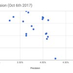
A recall / precision comparison of 1st generation models
2nd Generation
Artificial Neural Networks (ANNs) models automatically trained with BeagleML, an internal prototype for automated hyperparameter tuning.
Features and training set:
- Class balancing (SMOTE)
- 8 attributes selected from among 36 through Recursive Feature Elimination (RFE)
- No feature engineering
Free hyperparameters (ANN):
- Depth: 1, 2, 3 layers
- Neurons per layer: 40, 100, 200
- Learning rate: 0.1 - 0.001
- Activation functions: ReLU / Sigmoid
- Batch size: 50,000 - 10,000 samples
- Epochs: 50, 75, 100
Fixed hyperparameters:
- Optimizer: Adam
- Output function: Sigmoid (threshold = 0.5)
- Cut-out accuracy: 0.9
Technology used:
TensorFLow, Python.
Results:
Cognitive metrics were collected from 2,212 trained models.
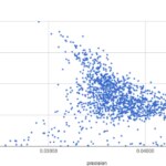
A recall / precision comparison of 2nd generation models
3rd Generation
Logistic regression models automatically trained.
Features and training set:
- Class balancing (SMOTE)
- 1 to 36 attributes selected from among 36 through Recursive Feature Elimination (RFE)
- No feature engineering
Free hyperparameters:
- Number of features: 1- 36
Fixed hyperparameters:
- (default values and parameters of libraries used)
Technology used:
SciKit Learn, Python.
Results:
Cognitive metrics were collected from 36 trained models.
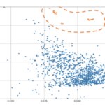
A recall / precision comparison of 3rd generation models (in orange) vs 2nd