The most common approach to neural network training in the academic community is based in dedicated hardware packed with an increasing number of more powerful GPUs. Probably acquiring a small number of these machines for research purposes is not a specially challenging task. But the purchase of a big number of them in a multinational financial institution can take a while. So a way to gather a similar amount of processing power with already purchased general purpose hardware can be appealing if the goal is to be agile and be able to respond to market needs fast.

Another limitation of having a small yet powerful machines is that it may not be possible to run many processes in parallel. It may be interesting to run more than one at the same time even if they are a bit slower.

The size of the data collected by modern systems makes the task of moving them to the dedicated hardware problematic. In that sense it may be a good idea to move the processing power closer to the data. This is the approach used in Spark and similar systems. Right now there are no good ML libraries on top of Spark.

Another point against the dedicated hardware is simple flexibility, the same general purpose hardware can be used for other purposes instead of sitting idle when no training is needed.

To achieve maximum flexibility and adhering to the distributed computing principles the software should be deployed in containers (docker, rkt).

The previous considerations leads to the idea of investing time in trying to see if it was viable the idea of using distributed neural networks. In this post we focus in one Machine Learning framework capable of doing it: Google’s Tensorflow.

The goal of the project was to develop an architecture as flexible as possible, it must be possible to run different kinds of models to solve different kinds of problems. So the systems must be as data agnostic as possible.

The system should not store data locally if possible. The rationale of this is again related with flexibility. This is against the actual trend of moving the code to the data. But there are cases where it may be a good idea, for example when the data comes in streaming. Banking operations or business events come in a stream. This approach can be useful to produce systems that are constantly learning from the live stream of events.

A machine learning system capable of learn in real time from a live feed of events, capable of scale to match the changing load of events is an appealing and challenging goal worth trying.

A machine learning system capable of learn in real time from a live feed of events, capable of scale to match the changing load of events is an appealing and challenging goal worth trying.

Architecture

The following describes the architecture tested at BBVA Labs, it is based in the Tensorflow framework although most of the concepts are also present in other modern frameworks. In general terms all the frameworks use this same approach.

The data scientist defines a model (algorithm) to solve a machine learning problem. The model can be programmed in several languages, the most popular these days are Python and R. These ones are simple to learn as Python or well suited for data processing like R but at the end they are not the best in terms of performance. The frameworks usually compile the source code into a mathematical abstraction, usually a graph that is later compiled using a lower level language capable of better performance. They use heavily optimized libraries, sometimes specific for each hardware type.

The following image is the representation of a neural network modeled as a graph. The screenshot is from Tensorboard, a tool included in the Tensorflow distribution that helps diagnosing problems in a model.

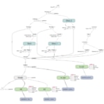
Having the operations represented as a graph makes it easy to calculate derivatives, for example.

How to split a neural network

There are two ways to split load of a neural network into several machines:

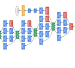
• Network / Model parallelism. Today’s neural networks are made of many layers. Each layer requires a set of computations that are usually represented as a graph. The data is passed along the calculation nodes of the graph in tensors which are just multidimensional arrays. For example an image can be made of 4 color channels (R, G, B, A) each of them being a 2 dimensional array (3 dimensions). If the input is a video we have a new dimension, time. If, for performance reasons, we pass more than one sample in a batch we add another dimension.
  In this approach each computation can be placed on a different device, a device can be a CPU or GPU on the same machine or in a different one. This way it is possible to get the best of each available device but it is needed to develop carefully and assign each operation to a specific device. This means that it is needed to know in advance the hardware the model will run in. This can work on a lab but it may not work well in an industrial / business environment.

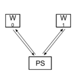
• Data parallelism. The whole model is run on a machine. Several machines run the whole model with different parts of the data. Each of the machines running the model is called a worker (W). Every given amount of time (usually after a batch) the different instances of the model share the parameters and reconcile them before continuing with the training. They send the information about the parameters to a set of machines called parameter servers (PS) that merge the results and send them back to the workers.
  This approach solves the problem of knowing the hardware setup in advance. In fact it can be changed at any time. This is a plus from the resiliency point of view. This can be very important in the case of very long computations. It also gives flexibility in the sense that it may be possible to increase or reduce the number of machines (computer capacity) to make room for more jobs. It also comes with a price. New machines are needed in the form of the parameter servers that will be in charge of gathering and merging parameters.
  The reconciliation process can be synchronous or asynchronous. Both have advantages and drawbacks. The asynchronous is more resilient and allows the usage of machines with different processing power but it may waste part ot the computation time. The synchronous one instead works better if all the machines have the same processing power and are close in the communication network. But it is more sensitive to any issue with the worker nodes. It also requires extra code to do the synchronization.

Environment

In order to evaluate data parallelism the following environment has been deployed. Not all the elements needed are described here, only the ones that have effect in the performance.

• Data: As explained, the data will not be stored in the processing machines, it will be sent to them. This way we simulate a probable scenario where the data is received in streaming. For testing purposes the data can be stored in files in specific (non processing) machines or generated by a botnet simulating the behaviour of customers.
  This setup simplifies the distribution of the data to a variable number of processing nodes. This is of course not the fastest way to process data in a machine learning environment.
  This task is done using a kafka cluster. The botnet publishes the events on a topic and the processing nodes acting as consumers read them and use them as input vector for the neural network.
• Processing: The training of the neural network in a distributed way using Tensorflow requires the use of two type of nodes. The work itself is done by the worker nodes. There is also a set of nodes (parameter servers) that receive the different versions of the parameters generated by the worker nodes and reconcile them before sending them back to the worker nodes. The parameter reconciliation is done in asynchronous mode.

All the elements are deployed as containers managed using Rancher. Each run with different settings is deployed in a stack. The use of Rancher allows to deploy hybrid systems where part of the nodes are deployed in a different cloud.

Key factors in terms of scalability

The main goal is to find out the limits in terms of scalability. Namely finding when adding more processing nodes does not produce an equivalent reduction in time. The way to test this a set of training runs with the same data but different settings, mainly different number of nodes. Once a limit is reached we change other infrastructure parameters to see how it affects the performance.

Neural network topology

The topology of the network, the number of layers and their size has a major impact in the performance. If all the network is to be calculated in the same worker with data parallelism it is important to ensure that it fits in a single machine. In the case of very big networks it may not be best solution.

Training batch size

As explained before, in data parallelization different worker nodes train using different parts of the data. From time to time it is important that the network parameters are reconciled (merged by average) to ensure that all converge to the same solution. Usually this happen after a number of training batches.

If the batch size is too big different nodes will drift away from the average and when the merge happen they will be moved back. Part of the time consumed will be wasted. On the contrary if the number is too small the merges will be more often and more time will be spent on the merging and communication process.

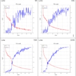
The following graphs illustrate this effect. They represent the same experiment involving 4 worker nodes and 2 parameter servers. The only difference in the batch size (50, 100, 500 and 1000). To ensure that the networks are not idle waiting for the data the botnet runs faster. That means that at the end they consume much more data and computing power when the batch is bigger. But it does not improve the final time to reach the top accuracy. The weights on each node drifts so much on each node that when the average is calculated they have wasted too much time. And it takes longer to calculate the model.

Data distribution

It is important to ensure that the data is properly shuffled otherwise it may be the case that certain worker nodes receive only certain type of data and the training of these nodes is constantly modified by others.

Data input

The bandwidth of the input network (handled using kafka in our case) can be a limitation if too many workers are present or if the input vector is too big. A big number of workers means that more data must be sent over the network to keep all the workers busy. This will be a limiting factor in the final throughput of the model. A way to overcome this is placing the data in the worker nodes in advance. But that is not the proposed architecture in this case.

The bottleneck can be caused by the network bandwidth itself or any component involved in the data distribution.

Variable distribution across the parameter servers

As explained before the coordination of the network parameters in the form of Tensorflow variables is done using the parameter servers (PS). Each variable is assigned to a server. All the workers will communicate with that server periodically to merge the value of the variable with the rest. It means that on startup all the variables must be assigned to a specific PS and all the workers must be aware of that. This assignment can be done manually by the programmer of the model or it can be done automatically by the device setter provided by the framework.

The manual assignment will probably give better performance but it can be done knowing in advance the hardware involved. The goal of this work is to study how to run neural networks in a flexible way so there is no point in manual assignment.

The device setter until version 0.11 did this using a round-robin strategy. The programmer must be aware of this to avoid falling into cycles where all the “heavy” variables fall into the same PS. This may happen more often than imagined.

For example: During the development of a deep neural network several layers have to be created. If these are fully connected layers they will have two variables, weight and bias. The first one will be at least two dimensional array and the bias will have one less dimension, making it maybe thousand times smaller that the weights. A natural way to create this is in a loop. Each pass will create a layer, creating the variables sequentially first the weight and then the bias. If there are only two PS the round-robin will assign all the weights to the same PS and the biases to the other.

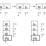
The problem can be easily solved adding another PS, but the operator must be aware of if all the time. In version 0.11 the device setter accepts a strategy function as parameter. The function knows the devices, parameter servers. Every time a new variable is created, this function is called and returns the device where it must be assigned. As of release of version 0.12 two strategies are provided, the first is round-robin which is selected by default. The second one is a greedy one that aims to spread them across the PS based on the size in bytes. The strategy must be greedy as it does not know the variables in advance. If the network has many small variables they may end all in the same PS adding extra pressure on it causing a bottleneck.

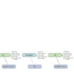
The following images illustrates how Tensorboard (Tensorflow’s approach to debug) shows the location of the variables in the devices. It can be seen that h0, h1 and h2, the variables that stores the weights of the matrix area all stored in the same parameter server. This can convert parameter server /job/ps/task:0 in a bottleneck.

Number of workers

This is the most obvious one. The system cannot scale to the infinite. A very big number of workers must be kept fed with input data and they must send the variables to the parameter servers.

As more workers are added the overall training time decreases but beyond certain point no improvement is noticed. It is better measured viewing the aggregated computation time that measures the total cost. As long as it remains flat the addition of worker nodes is cost effective.

There is a sweetspot for each model. It is not the same in all the cases. During the tests some models reached it at 7 and others at 20. But in complex models (millions of parameters due to very big images for example) the number can be much bigger.

Number of parameter servers

As explained, the variables storing the network parameters are kept in the parameter servers. If the number of them is too small the load on them will be too high. In the test runs they end up using all their network bandwidth. The initial upper limit seems to be one parameter server by variable but this will not be cost effective.

Two ways to handle this limitation have been identified but not tested. If the execution is done in a cloud infrastructure it may be a good idea to use machines with the highest bandwidth available. The Tensorflow documentation states that variables can be split and stored in different parameter servers. This can be used in the case of a very big variable, to share the load among the parameter servers.

It is important to note that all the workers must communicate with all the parameter servers every merging cycle.

We have also found that the first two parameter servers (0 and 1) also store variables related with the saving of the session. This of course impacts on the network bandwidth consumed by them. It may be worth trying a strategy that stores the variables in other parameter servers different that 0 and 1.

Communication network topology

As explained in the previous points the communications in general can be a major bottleneck and must be reviewed carefully. As stated it is important that the parameter servers have the best network connectivity as they will receive information from all the worker nodes.

The distributed approach in general is specially appealing for cloud environments. The type of the machine is important, the affinity of the containers must be set carefully.

Conclusions

Distributed neural networks cannot be scaled to the infinity. Despite the claims of Google that they can scale to the thousands, it may need a very careful design not suitable for generic use.

Distributed neural networks cannot be scaled to the infinity.

Different elements have different needs in terms of network and processing power. If a cloud environment is to be defined, it may be a good idea to use different kinds of hardware hosts. The worker nodes need mainly processing power and probably RAM. If they have GPUs the performance can be enhanced greatly. But it is important that all nodes have similar characteristics. In the case of the parameter servers processing power is not so important but network bandwidth is critical.

In the case of hybrid cloud environments or clouds distributed in several locations, it is important to ensure that the workers and the parameter servers are not far enough in terms of latency and bandwidth.

The usage of nodes with dedicated GPUs increases the performance greatly but it comes with cost of specific development. From the Tensorflow point of view it’s just a matter of setting the device. But in a distributed environment the hardware must be perfectly known in advance or some specific code must be included in the model to discover the available hardware. Even this can be problematic, because slower nodes can reduce the performance or its calculations completely ignored.

An important limitation in Tensorflow is related with scalability. On startup time, all nodes must know the IP addresses and ports of all the nodes in the network. It means it cannot scale up on the fly. It can scale down, if a worker node goes down the network keeps working fine. This is good from the resiliency point of view. If more nodes are needed the processing must be stopped, the new nodes are added and the network restarted. The work already done until the pause will not be lost if the session is saved. This is fully supported by all frameworks including Tensorflow but the model must be programmed taking into account this possibility.

In conversations with a Google engineer, he said it was possible to add redundant workers that remain idle until some node fails, keeping the expected performance in the case of data parallelism, or preventing error in the case of a model divided between different machines, but this was not tested.

We encourage you to send us your feedback to BBVA-Labs@bbva.com and, if you are a BBVAer, please join us sending your proposals to be published.